Working with Point Clouds
Pre-processing, managing and attaching point clouds
To pre-process a point cloud, use the POINTCLOUDREFERENCE command to open the Point Cloud Cache Manager dialog box, then select Process a file or Process a folder. You can also use the POINTCLOUDATTACH command.
You can start pre-processing a point cloud from a saved or unsaved DWG file. You are asked for the input point cloud (no units or insertion point).
All data is read, processed and written to disk, and a LOG file is created. The progress is tracked and shown in the Point Cloud Cache Manager dialog box.
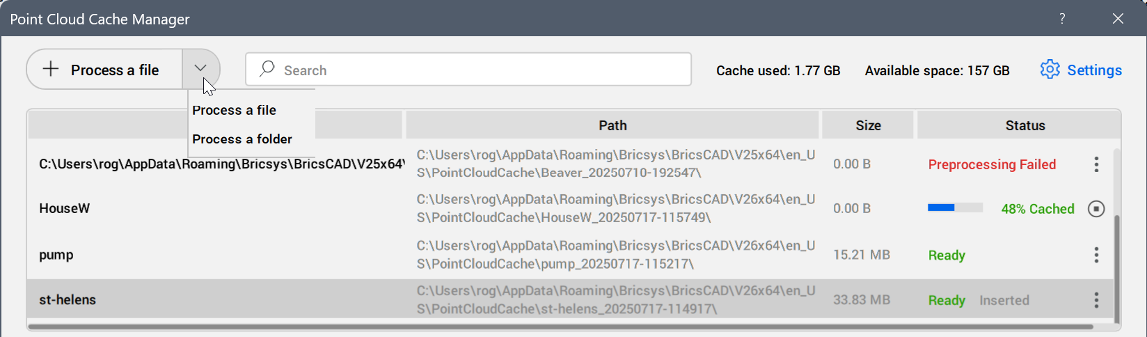
Pre-processing point clouds has two steps. The first step is processing the points, and the second step is visual optimization.
The point cloud files and the 360 images are made available almost instantly in the drawing, with the bubbles displayed in purple. These bubbles do not contain information such as normals and depth per points. The bubble pre-processing continues in the background until all the information is ready. The bubbles are then displayed in green.
The progress of the pre-processing is recorded in a log file in the sub-folder related to the point cloud. This sub-folder is located inside the current point cloud cache path (can be set in the POINTCLOUDCACHEFOLDER system variable). The default path for the current point cloud cache is C:\Users\%username%\AppData\Roaming\Bricsys\BricsCAD\V26x64\en_US\PointCloudCache\Folder_for_processed_pointcloud.
- Search for a file or filter the list of cached point clouds with the search bar at the top.
- In the Details section, see all metadata available for the selected point cloud.
- You can edit the data name, the unit and the GIS coordinate system.
- Any subfolder with previously pre-processed point cloud cache data (from another BricsCAD point cloud cache folder or pre-processed with the shell executable preprocessor.exe) can be copied in the folder specified by the POINTCLOUDCACHEFOLDER system variable (default value: C:\Users\%username%\AppData\Roaming\Bricsys\BricsCAD\V26x64\en_US\PointCloudCache). The cache files will be available next time you open the Point Cloud Cache Manager dialog box. For each subfolder in the point cloud cache folder, there is an item in the Point Cloud Cache Manager dialog box.
- If a point cloud cache of a file processed in HSPC format is not found at the specified location, a tray notification redirects you to the Attachments panel. From here you can select a new path for the cache folder.
To start the attachment of a cached point cloud, use the Attach button. The Attach Point Cloud dialog box opens. Here you can set the insertion point, scale, rotation, unit, and GIS coordinate system of the point cloud instance. You can also decide to use the geo data (if available).
Alignment
The POINTCLOUDALIGN command automatically rotates a point cloud to optimally align it with the X and Y axis, taking into account the vertical planar surfaces in the point cloud (e.g. walls). To determine the best alignment, you are asked to specify the most relevant area of the point cloud containing walls.
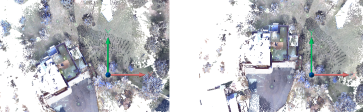
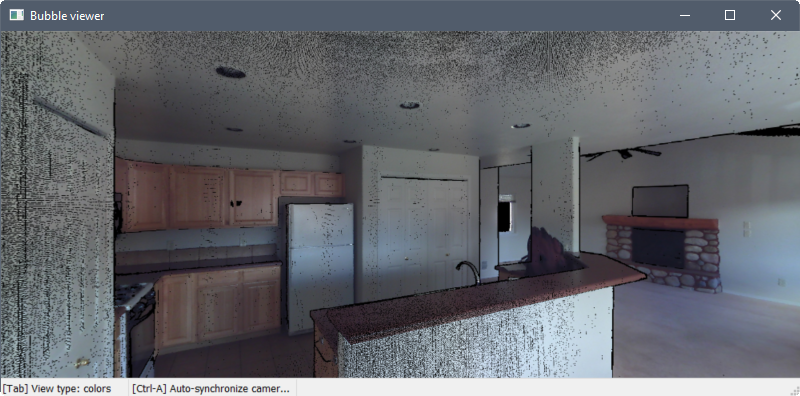
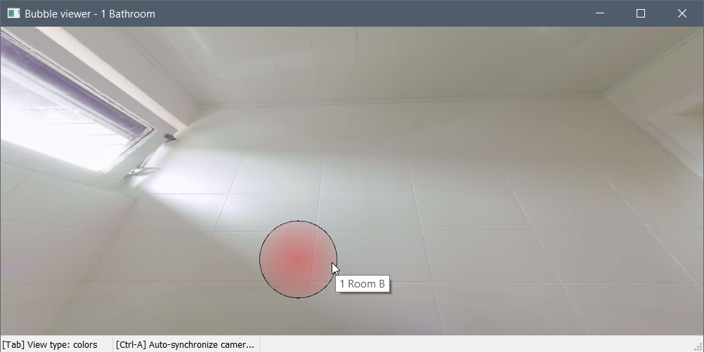
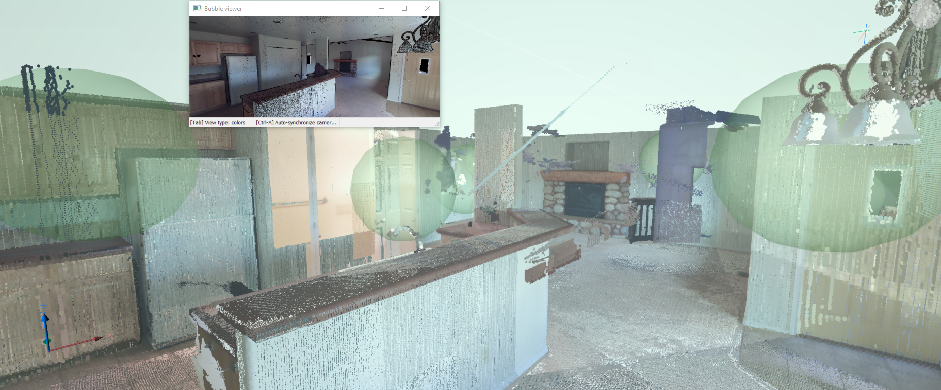
Bubble Viewer
Depending on the original file format of the point cloud and the type of scanner used during scanning (static or kinematic), bubbles (green spheres) or waypoints (blue spheres) might be shown at all the scan locations. At these locations, you can experience the most realistic visual representations by opening the Bubble viewer.
To open the Bubble viewer:
- Run the POINTCLOUDBUBBLEVIEWER command.
- Select the Open scan in bubble viewer option from the context menu of scan or waypoint listed in the Point Cloud Manager panel's Scans or Waypoints lists.
Structured data is captured using a static scanner. In this case the location of the scanner is known for every point. Green bubbles are created at the locations of the static scanner from the scanned points.
Unstructured data is captured using a kinematic scanner. In this case there is no exact location from where the points were scanned. Some of the kinematic scanners create panoramic images at time intervals. For these images the location is known and waypoints (blue spheres) are created.
Indicate a bubble index in the POINTCLOUDBUBBLEVIEWER command or double-click one of the bubbles in the model space to open the Bubble viewer.
Press and hold the middle mouse button and move the mouse to view the point cloud in any direction from that scan location.
Zoom in and out using the mouse wheel.
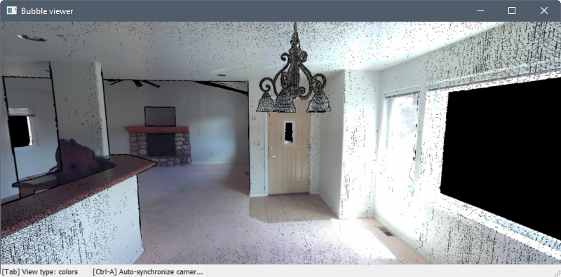
Nearby scans are indicated in the Bubble viewer by red bubbles. Hover the cursor over a bubble to display the scan name. Double-click a bubble to open the scan in the viewer.
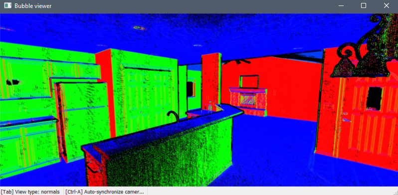
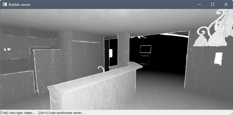
Press the Tab key to cycle through three different visual modes (view types).
-
The colors and colors (depth) modes display the points as their actual colors or in grayscale, depending on how the data was scanned.
-
The normals mode displays the points as red, green, or blue according to their normal vectors. The colors correspond to the UCS axes.
-
The distances mode displays the points from light to dark as the distance from the scan location increases.
Sync the drawing view to match the Bubble viewer by pressing Ctrl+A.
Entity snaps
The Point Cloud Nearest Point entity snap (PCNEAREST command/3DOSMODE system variable) significantly improves the ability to select relevant point cloud points. It uses an imaginary cylinder from the current viewpoint toward the cursor.
The radius of the imaginary cylinder is defined by the Entity snap aperture box setting (APBOX system variable).
Turn on the Point Cloud Nearest Point entity snap (bitcode 128 of the 3DOSMODE system variable) together with other 3D entity snaps in the entity snap menus, toolbar and settings.
Export
The POINTCLOUDEXPORT command allows you to export the visible parts of a point cloud to a PTS, HSPC, or LAZ file.
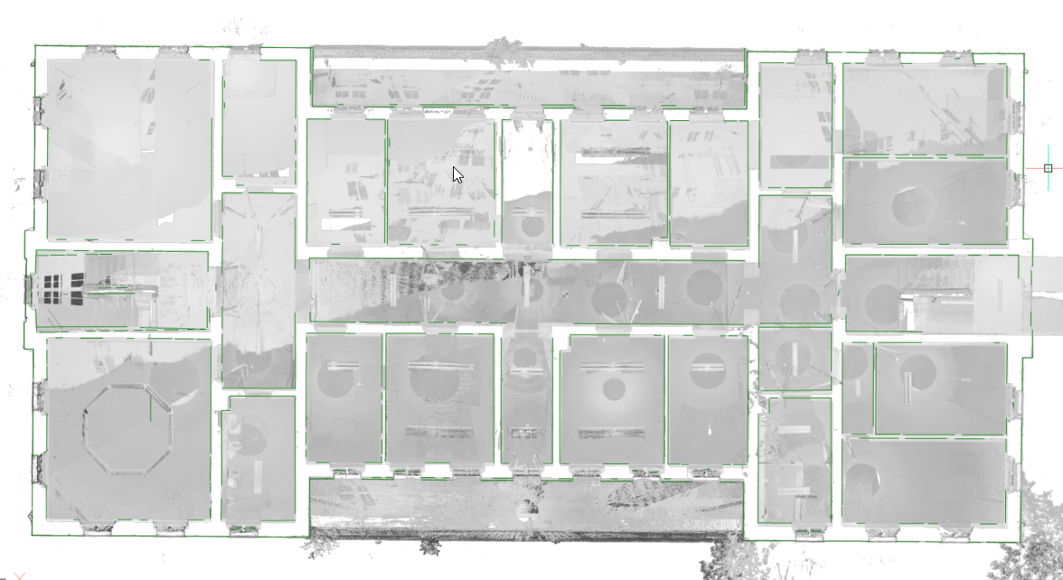
Floor Detection
The POINTCLOUDDETECTFLOORS command detects floors in a point cloud of a building. The detection is based on regions of points with similar Z-coordinates. The detected floors can help in navigating point clouds of buildings.
- For a better floor detection process, hide the points that are not related to the building (environment, other buildings, etc.). You can use point cloud commands like POINTCLOUDCROP, POINTCLOUDREGION, POINTCLOUDCLASSIFY. Turn off the visibility of the non-relevant classes in the Point Cloud Manager panel.
- The POINTCLOUDDETECTFLOORS command is used as a step in the point cloud Scan to BIM workflow. See the article Point cloud Scan to BIM workflow.
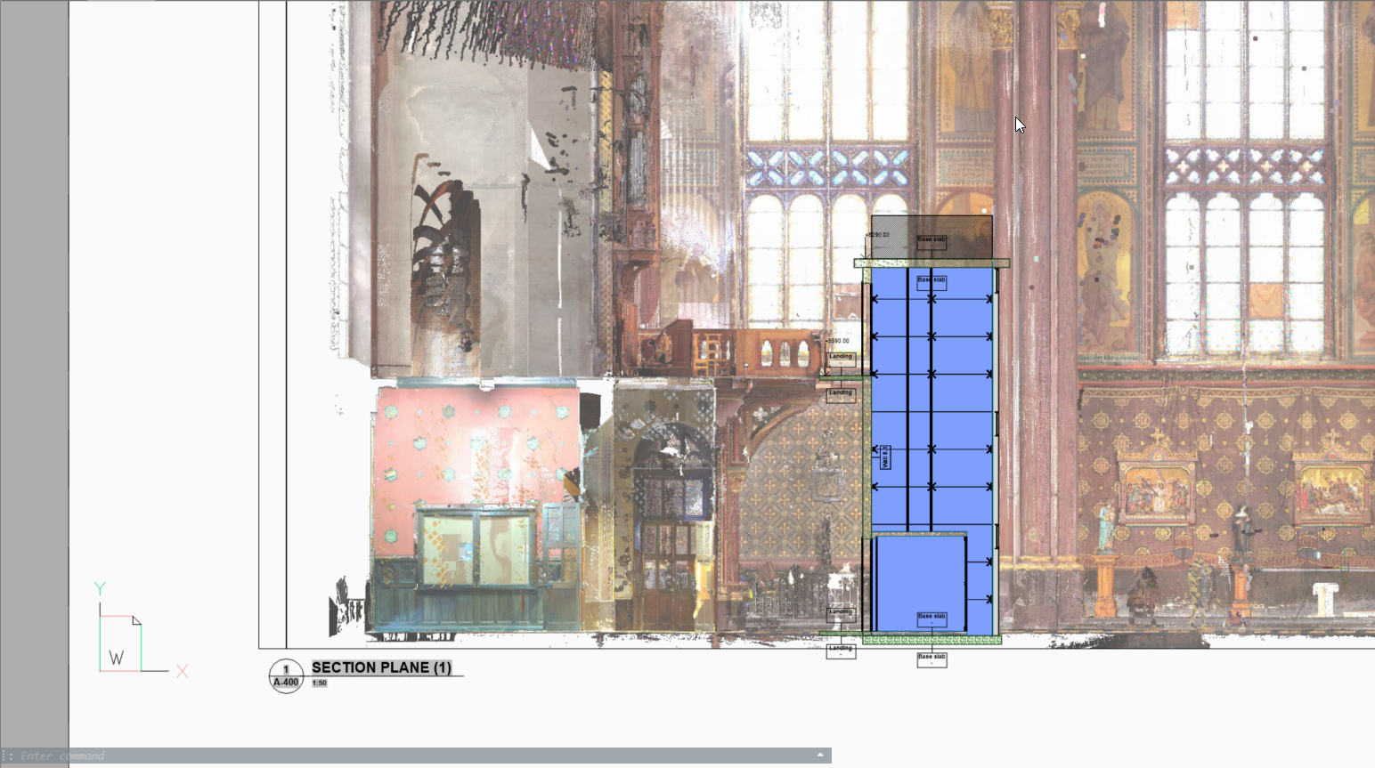
Point cloud projection
The POINTCLOUDPROJECTSECTION command enables you to detect walls from the volume section of a point cloud based on a variety of wall detection options. You can create volume sections with the BIMSECTION command. You can use these sections to generate 2D lines to create a 2D floor-plan or a vertical section. This is a background process and multiple sections can be processed in a queue. This way, it is possible to run this command in full resolution on all sections.
At the same time, a raster image is generated to give the user some context. In some cases, it is not necessary to recreate the existing building. Background images can give much more context to the design documents. These can be used to verify the created 2D geometry but in high quality scans, these images can also be used as graphical material. For example, as a background image for a BIM model in renovation projects where modern intervention are made in historical buildings.
Planar fit
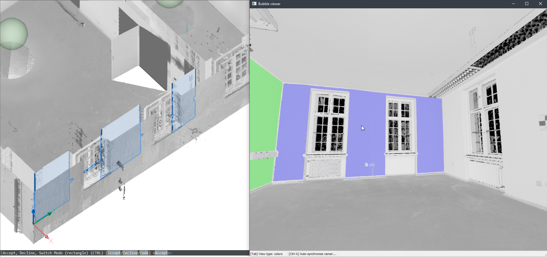
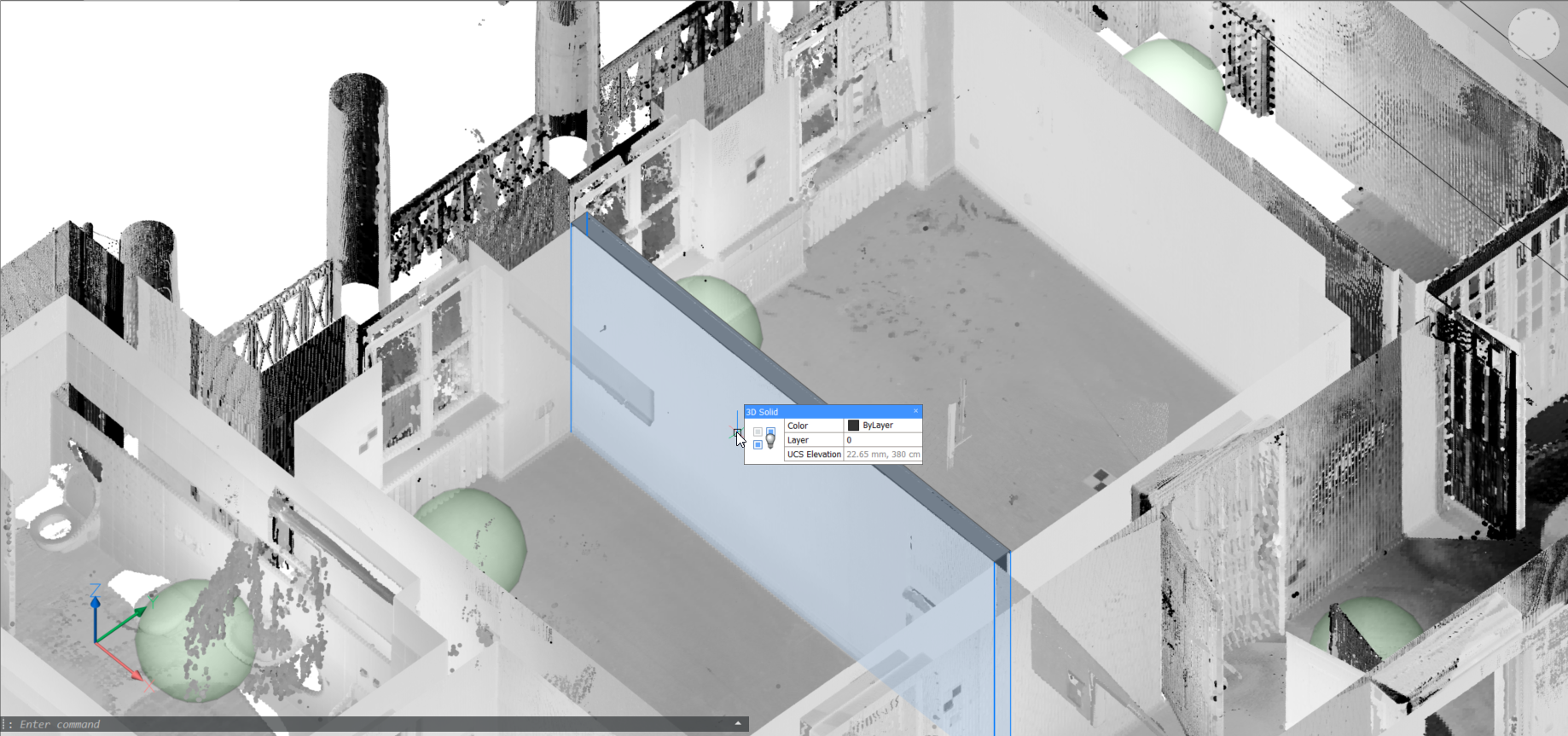
The POINTCLOUDFITPLANAR command enables you to create 3D geometry based on the point cloud. It creates a planar surface or solid after selecting a seed point in a point cloud. To detect the points that lie on the same plane as the seed point, a threshold value is used that can be set as a property of the point cloud entity. By holding down the Shift key and selecting the adjacent walls of a room, the fitted planes are extended/trimmed to form a closed surface.
- Select openings allows you to take into account the openings of doors and windows (only in Bubble viewer).
- Adjust borders allows you to adjust the planar border contour.
- Stitch surfaces provides stitching the result of multiple fitted planes into, for example, a solid which can be later used with the BIMINVERTSPACES command.
- In bubble view
-
If the Bubble viewer is open when the command is launched, BricsCAD expects you to select the plane seed points inside the Bubble viewer. The cursor gives you a preview of the normal direction of the plane. Next, you get a preview in both Bubble viewer and model view. You can toggle between the two shape representations using the Ctrl key.
Note: While still in selecting mode, the corresponding points in the bubble are shown in purple. These points are shown in green once the user accepts the generated result.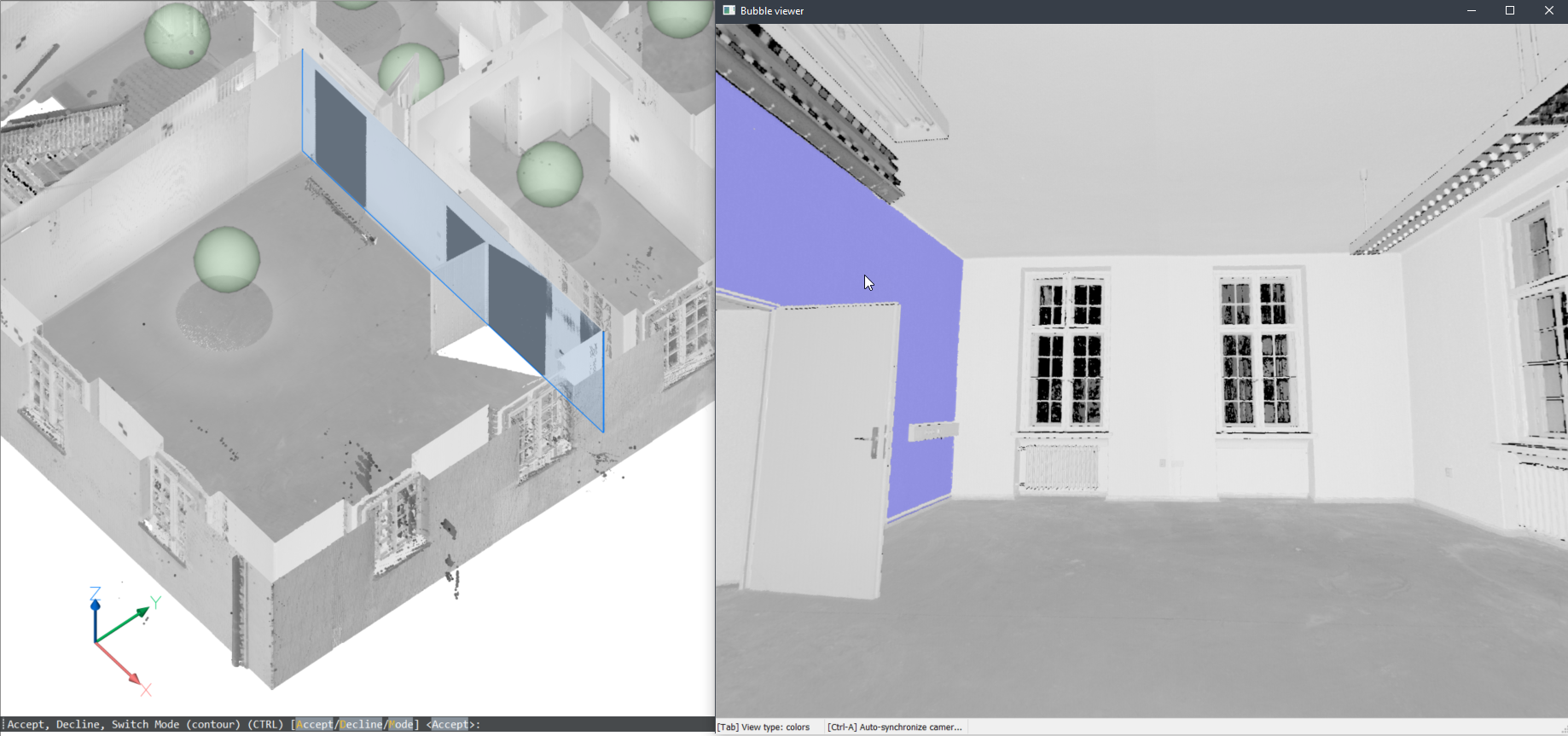
- In model space
- You can also use this command in the model space when the Bubble viewer is not open. BricsCAD asks you to select a point of the point cloud in model space. Depending on the size of the visible parts of the point cloud, this might take more time compared to running the command inside the Bubble viewer. However, this has two advantages by searching multiple scan positions:
- It can create larger surfaces by combining parts of different scans.
- It can detect wall and slab thickness.
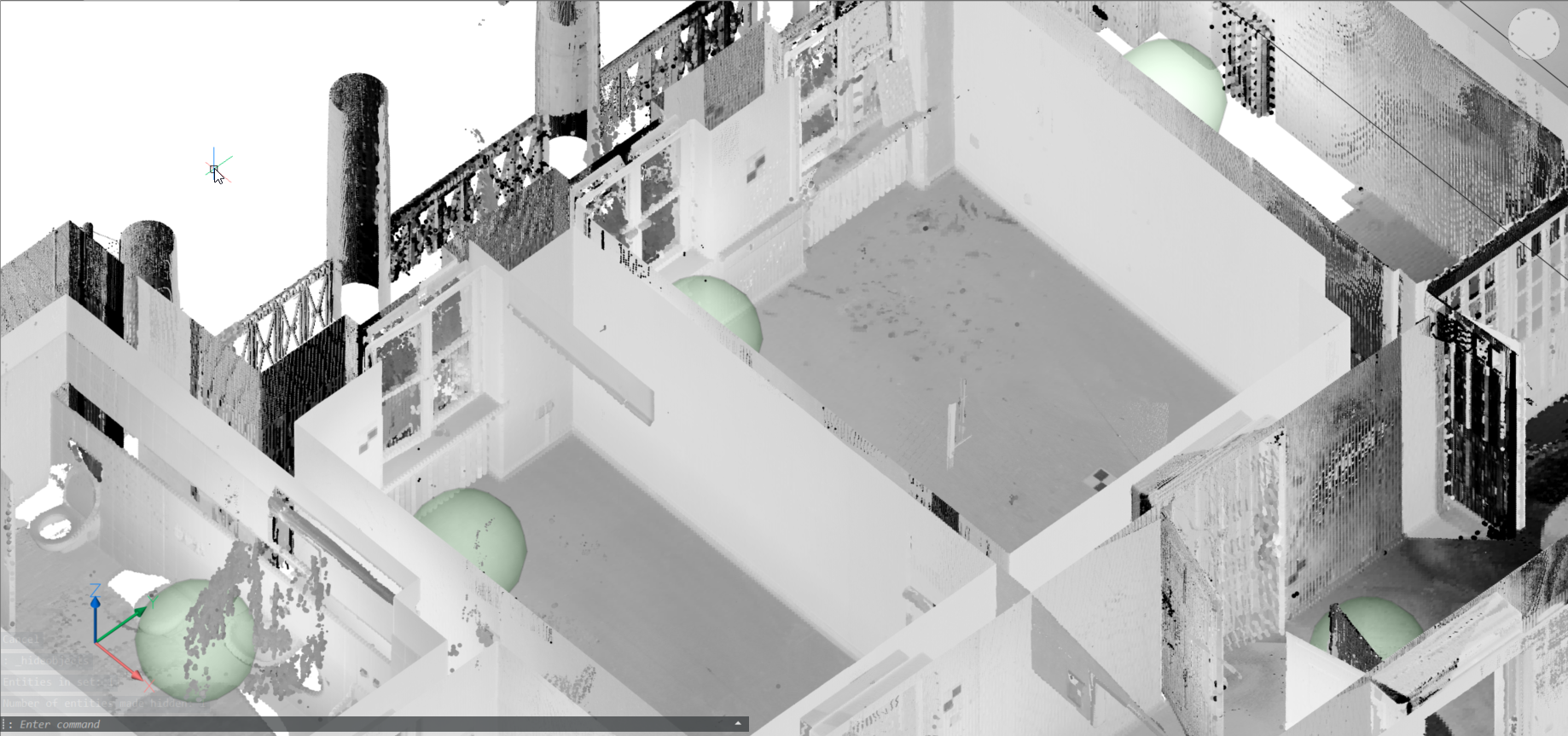
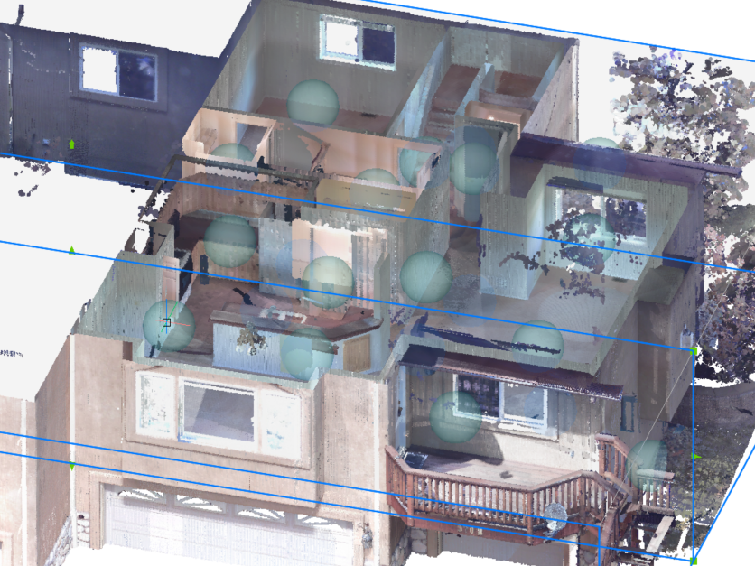
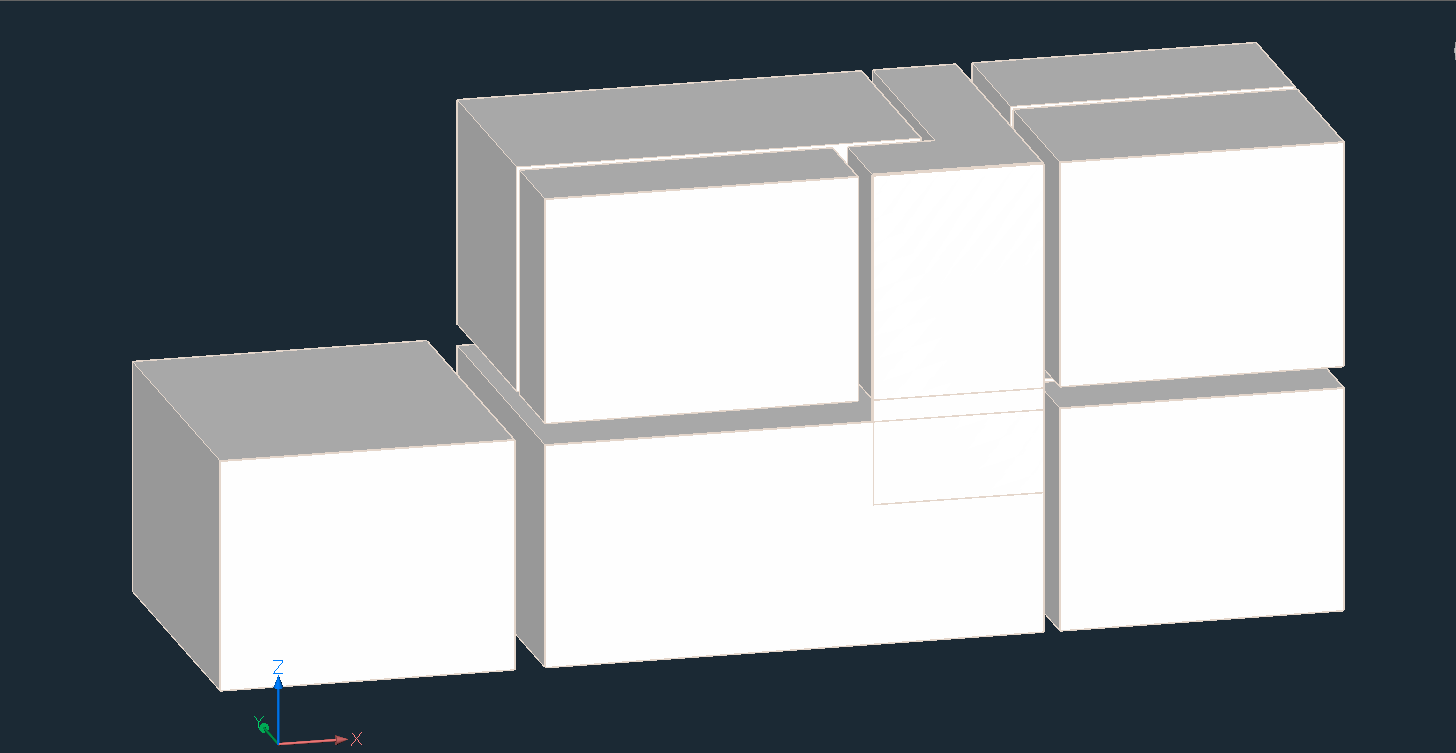
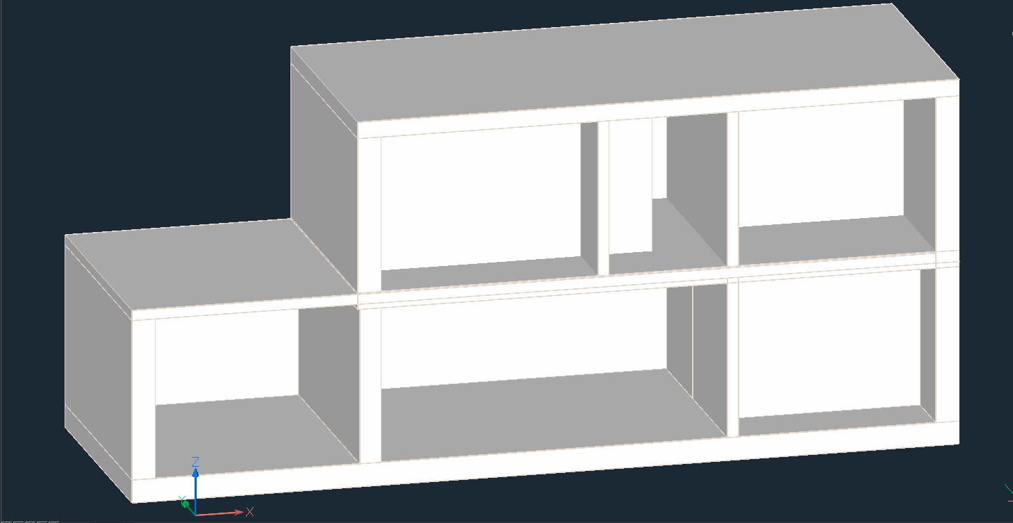
Note: Here, a work-flow of converting a scan to building model is provided. The point cloud (top image) is first converted to a set of solids, one per room, using stitched POINTCLOUDFITPLANAR results (middle image). The command BIMINVERTSPACES converts these temporary room solids into a building model with walls and slabs from the inversion of these solids.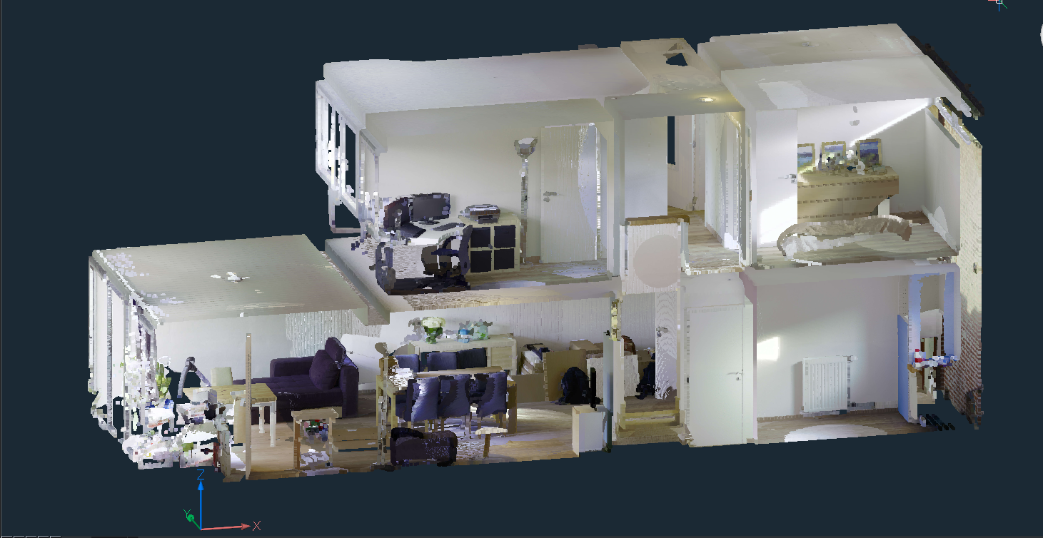
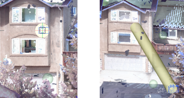
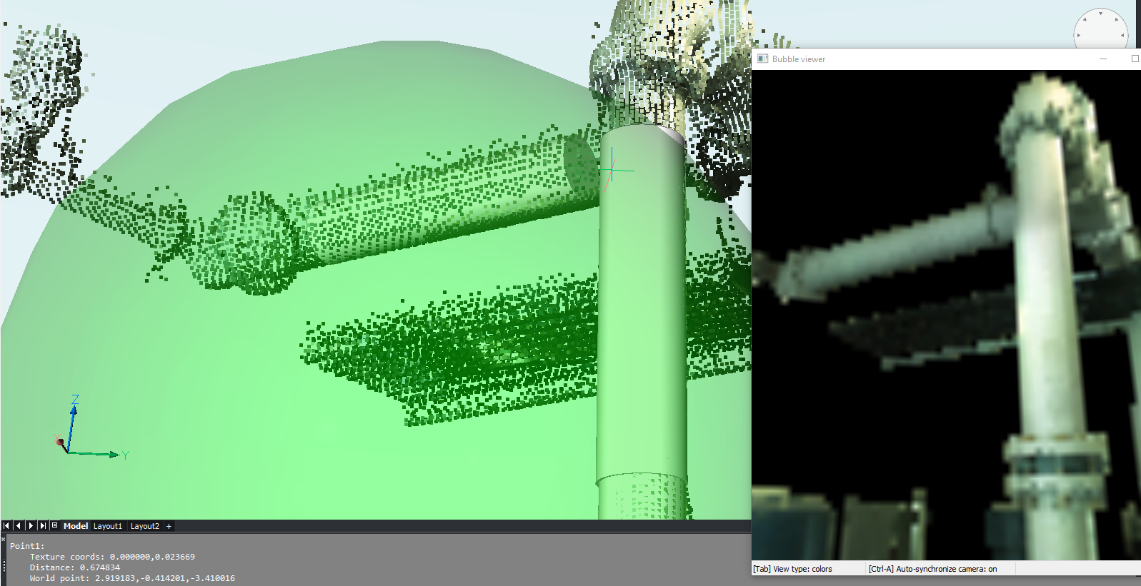
Fit cylinder in bubbles
By using the POINTCLOUDFITCYLINDER command inside the Bubble viewer, you can fit a cylinder to the cylindrical parts of a point cloud (for example pipes). Two clicks along the cylinder axis in the Bubble viewer are needed to extract a cylinder (a solid is created in model view).
POINTCLOUDDEVIATION
- The POINTCLOUDDEVIATION allows you to visually assess the fit between planar structures and points of the point cloud.
- Point cloud section of a floor of a house and a fitted plane:
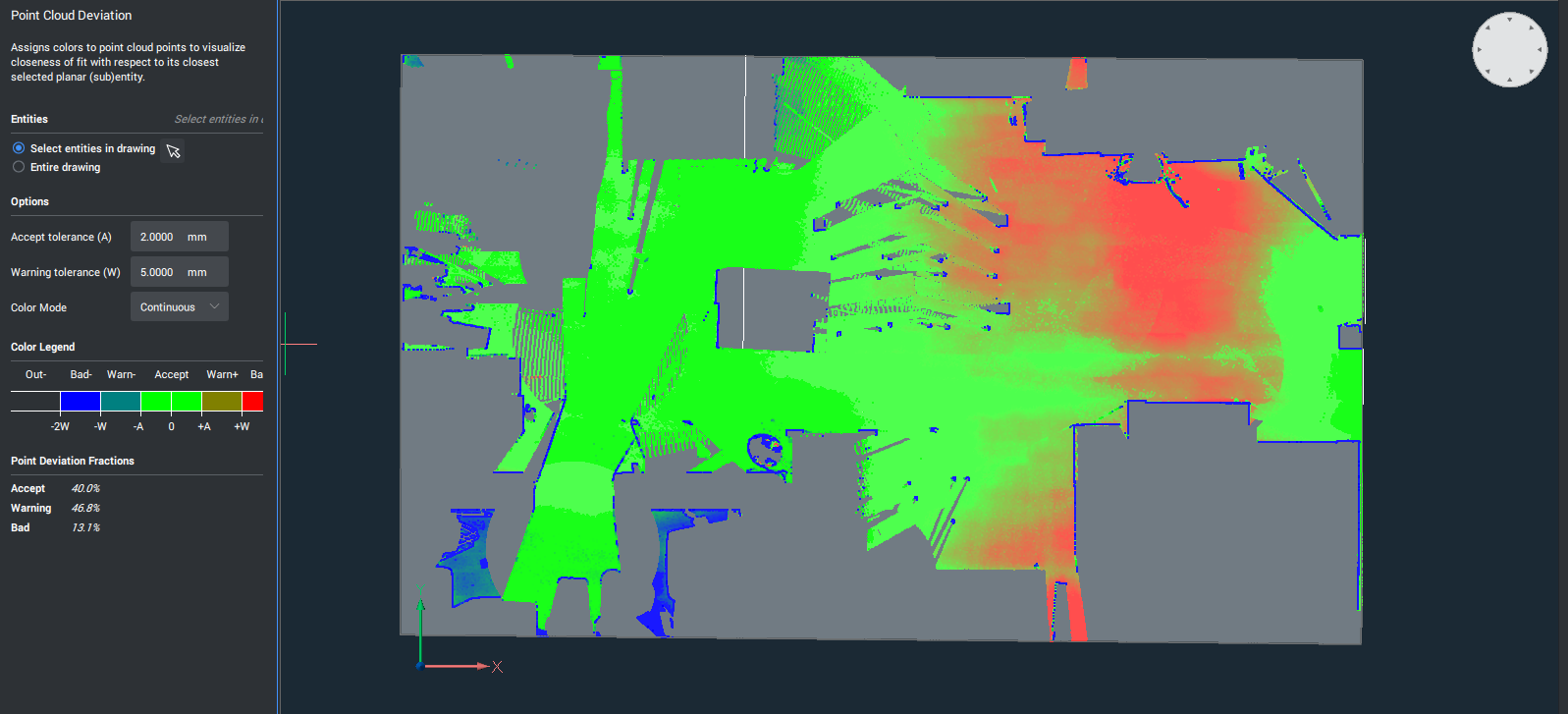
The distances of points from floor to the fitted plane are visualized using a colormap. In the left panel, an explanation of the colors is provided (green is planar, gradient from green to blue here is further above the plane, gradient from green to red is further below the plane). Also, a summary of the percentages of points in which category is presented (OK, warning level, …)